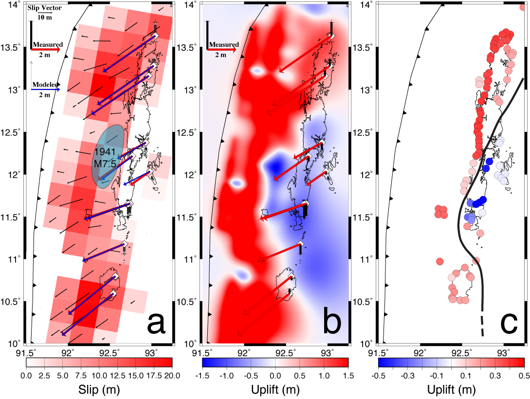
Figure 2. Coseismic deformation of the Andaman segment. (a) Red patches are a minimum-moment estimate of fault slip from 10 sparse GPS measurements (red/black = horizontal/vertical displacements). Blue/grey vectors are model displacements; blue patch delineates a 1941 M7.5 rupture. (b) Uplift predicted by the model in (a). (c) Conservative estimates of shoreline uplift derived from satellite imagery and tidal modeling by Meltzner et al. [2006]; the black line approximates an axis of neutral uplift.

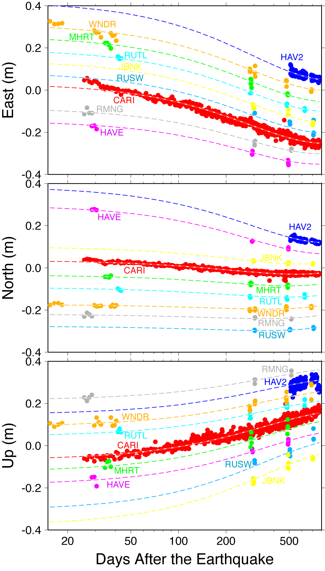
Figure 3. GPS displacement versus log-scaled time since the earthquake. Circles are GPS measurements; dashed lines are best-fit of an exponential function plus an interseismic velocity.

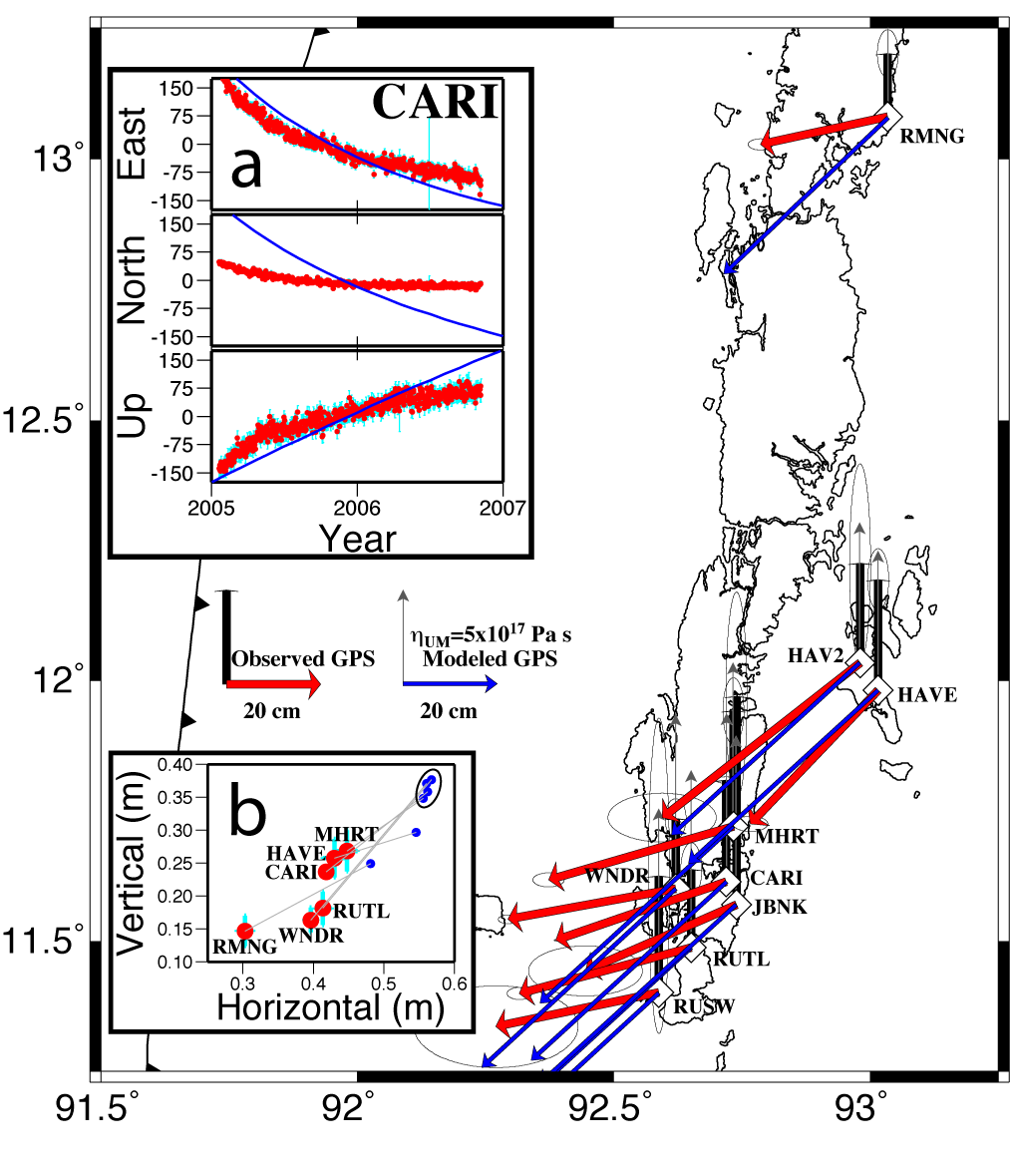
Figure 4. GPS-observed and viscoelastic-modeled postseismic displacements. Red vectors/black bars are 2004.98-2007.0 horizontal/vertical displacements, respectively, from exponential fit of the GPS data, with scaled 95% confidence ellipses. Best-fit model of viscoelastic relaxation, depicted as blue/dark grey vectors, assumes an elastic layer thickness of 70 km over a 5x10¹⁷ Pa s viscosity mantle. Inset a shows comparison of CARI GPS coordinates (red circles) to best-fit model (blue line). Inset b shows vertical versus horizontal transient displacement; red is GPS estimate (with 2s error), blue is viscoelastic model. Predictions for South Andaman sites are circled.

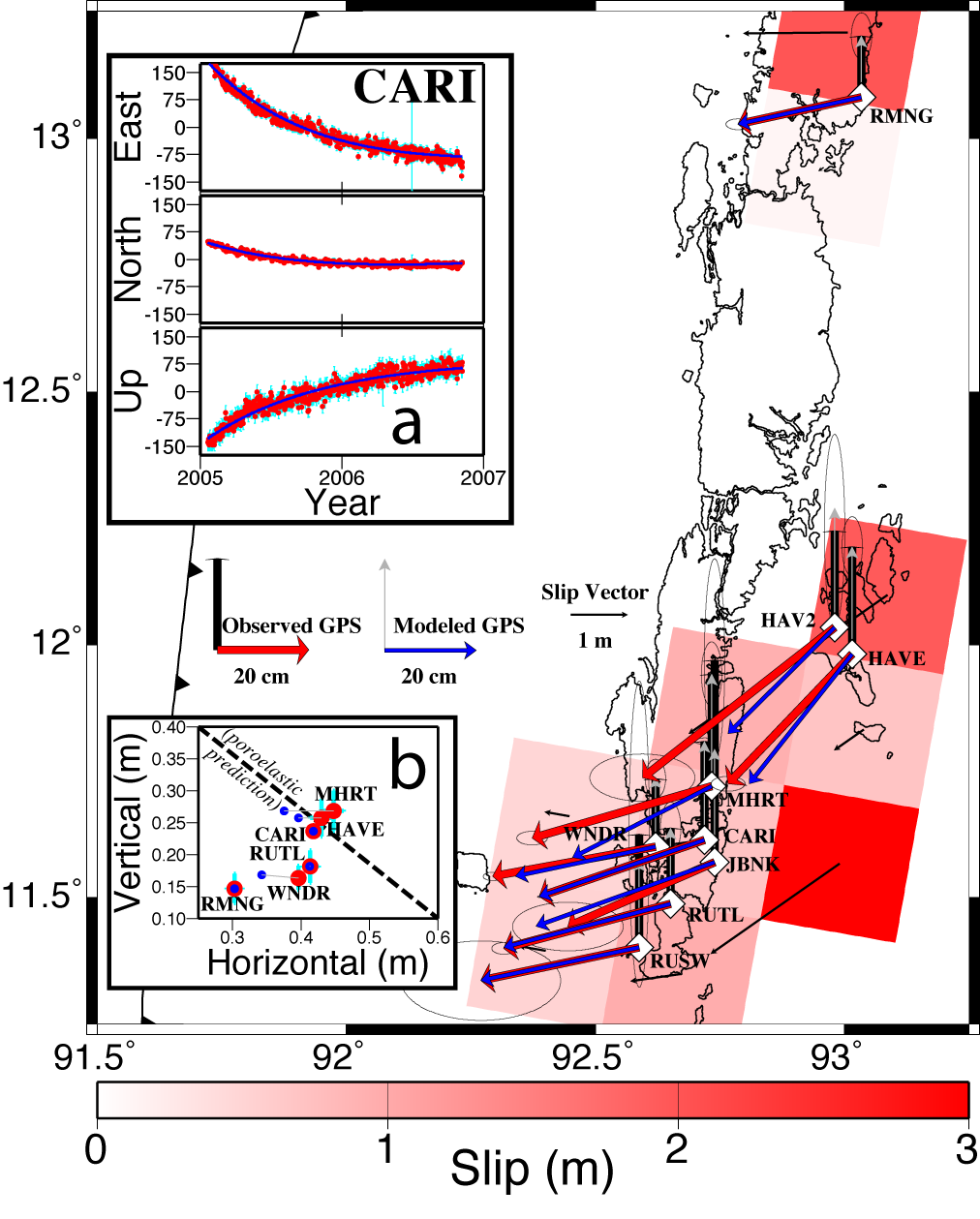
Figure 5. Andaman data modeled as slip on the subduction thrust. Red vectors are 2004.98-2007.0 displacements from exponential fit of the GPS data, with scaled 95% confidence ellipses. Blue vectors are the best-fit model of postseismic slip. Red patches with thin black vectors indicate the magnitude and direction of modeled slip. Inset a compares CARI GPS coordinates (red circles) to best-fit model (blue line). Inset b shows vertical versus horizontal transient displacement; red is GPS estimate (with 2s error), blue is slip model. Dashed line schematically shows negative slope of poroelastic response.

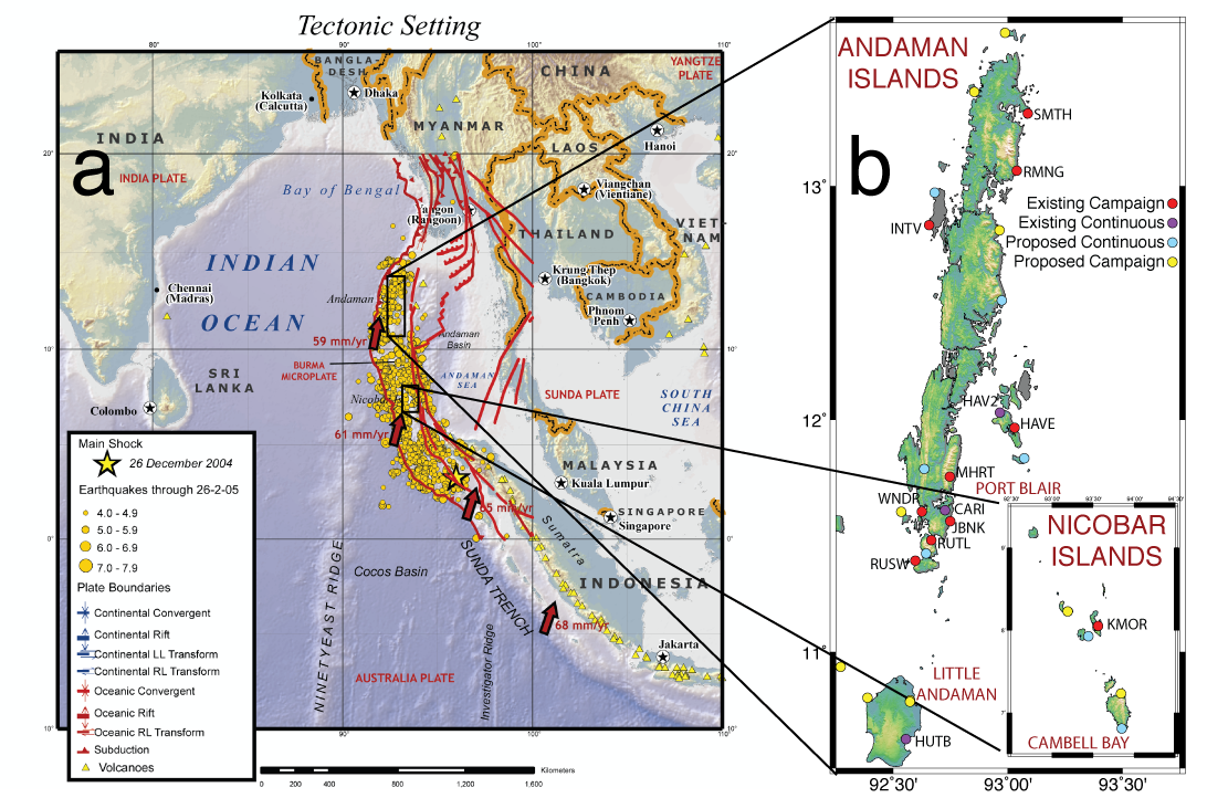
The December 26, 2004 Sumatra-Andaman earthquake (Figure 1) was the third largest earthquake of the last century (moment magnitude M_w = 9.3), and the second most deadly (~280,000 casualties). Seismic data suggested small (~1.5 m) amounts of rapid-rupture slip and moment release equivalent M_w~8.2 in the 500 km segment surrounding the Andaman Islands, but longer period seismic data and coseismic GPS displacements indicate average slip ~10 m within a ~100 km wide zone and moment release nearer M_w = 8.6 for the same region. Figure 2a shows a minimum-moment solution (also M_w = 8.6) for coseismic slip from the sparse available GPS data. Uplift at a local tide gauge occurred 20-30 minutes after passage of the rupture front, confirming that most of the Andaman moment release took the form of a huge slow slip event. The slowing of rupture in the Andaman segment is poorly understood, but may have very important implications for earthquake hazard globally.

Shortly after the earthquake, John Paul and Bob Smalley of the University of Memphis-CERI received NSF exploratory funds to measure subsequent movements of the Andaman Islands. Locations of GPS sites John installed for that purpose are shown relative to the regional tectonics in Figure 1 above. In the two years beginning 20 days after the mainshock, continuous site CARI moved 7.5 cm south, 31 cm west and rose ~23 cm. The campaign sites all exhibit similar uplift and SW to WSW motion, but magnitudes vary from 34 to 48 cm and azimuths differ by as much as 36 degrees. Transient motion is well approximated by exponential decay superimposed on an interseismic velocity, as illustrated by plotting the displacements (and their function fits) versus log of time (Figure 3).

Three processes have been identified as likely candidates for driving postseismic deformation: (1) poroelastic relaxation of stress as pore fluids flow from high-pressure to low-pressure zones created by earthquake strain; (2) viscoelastic relaxation by mantle flow in response to the coseismic stress change; and (3) aseismic slip in zones of "stable" friction within or downdip of the coseismic rupture. Surface deformation resulting from these processes can look very similar, suggesting that the effects of one process can be mismodeled using the physics of another. Laboratory deformation experiments indicate that all three processes should contribute to transient deformation following earthquakes, but the relative magnitude of each contribution should depend on the temporal and spatial scales examined. However examples of great earthquake postseismic deformation sampled densely in both time and space are few. Consequently questions remain as to the roles of these three processes in the earthquake cycle, and even whether they play a similar role on all fault zones or in subsequent events on the same fault zone.

We modeled the GPS measurements independently as both viscoelastic flow and fault slip on the subduction interface. The best-fitting model of viscoelastic flow (Figure 4) matches the data very poorly, and careful inspection of the measurements reveals that no physical parameterization can reasonably be expected to match the data. First, the timescale parameter of the exponential decay (t = 0.8 years) would require an extremely low average viscosity for the mantle (h ~ 7x10¹⁶ Pa s). An argument can be made that such extremely low viscosity is possible given an extremely high strain rate e^·, because effective viscosity in power-law creep varies proportional to e^·(1-n)/n. However the corresponding model displacements after two years vastly overpredict the measurements unless the elastic lithosphere is assumed to be extremely thick and/or flow occurs within a relatively narrow channel. Moreover, GPS sites on South Andaman are spaced only 10-25 km apart, but their vertical displacements vary by up to 40%. The spatial wavelength of vertical response to a deformation point source is roughly equal to the depth, and spatial wavelengths of viscoelastic response are filtered twice: once to propagate stress changes from the fault dislocation to the depth of ductile creep, and again thence to the surface. The temperature structure for subduction of 100 Myr-old oceanic lithosphere would preclude ductile creep above 80 km depth in this region, and the 70 km elastic lithosphere assumed in our best-fit model predicts only 7% variation in the vertical response of South Andaman sites (circled in Figure 4, inset b). These observations lead us to conclude viscoelastic relaxation does not dominate the first two years of Andaman near-field deformation.

The best-fitting model of fault slip (Figure 5) approximates the observations much more closely, with misfit error about one-tenth that of the best viscoelastic flow model. This is possible in part because the strain sources are at a depth of ~35-45 km, so large changes in the vertical response are feasible on distance scales of a few tens of km. Inset b of Figure 5 also shows that poroelastic response is an unlikely candidate for the Andaman deformation: Poroelastic models [e.g., Fialko, 2004] predict maximum uplift associated with positive coseismic dilatational strain, and subsidence with contractional strain. Horizontal motions are away from the uplift and toward subsidence, vanishing where vertical displacements are largest and maximal between a fluid source and sink where vertical displacement is 0. Hence, on a plot of vertical versus horizontal displacement, the distribution of measurements should have negative slope. The GPS measurements exhibit a positive slope distribution.

The postseismic fault slip model is intriguing for several reasons. Estimates of slip magnitude and relative contribution of strike slip both increase with depth, mirroring the surface GPS displacements, which are smaller and more trench-normal at western sites (Figure 5). Postseismic moment release is equivalent to a M_w > 7.5 earthquake, or about 10% of coseismic, and is probably larger given that only a small fraction of the Andaman segment is sampled by data presented here. 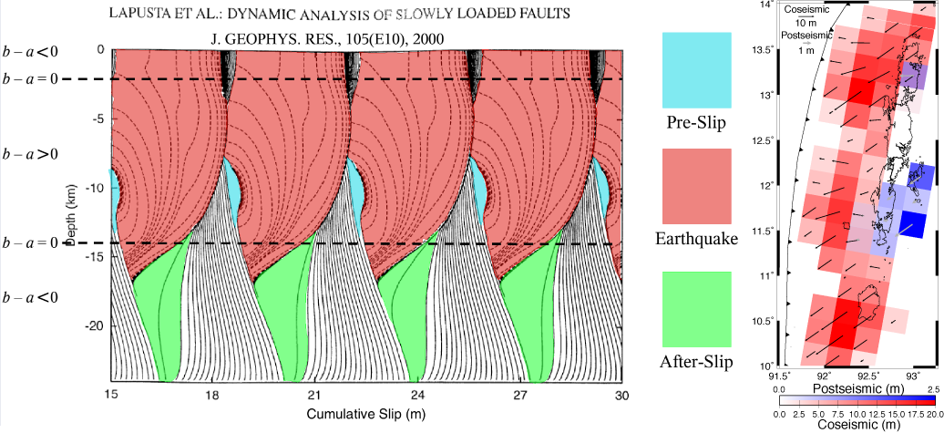Postseismic slip overlaps slightly with the coseismic slip estimate (Figure 6), but most of the moment release is further downdip. This pattern mirrors simulations of coseismic and postseismic slip in elastodynamic models of rate- and state-dependent friction [e.g., Lapusta et al., 2000], in which slip deficit accumulates in velocity-strengthening conditions during interseismic periods and catches up to coseismic slip over several years' time. Andaman data prior to 2004 are insufficient to assess interseismic coupling where we now identify postseismic slip. However modeling of interseismic slip and stress rates from GPS data at the Cocos-North America subduction boundary suggests locking above the frictional transition buffers stress accumulation in the shallow velocity-strengthening regime [Lowry, 2006], thus enabling slip deficit to accumulate that can drive slip following an earthquake.