Modeling and Inversion of Guerrero GPS Data:
Motivation:
| The Guerrero segment of the Cocos-North America plate boundary, between Acapulco and Zihuatanejo, is one of only two segments that has not experienced a shallow interplate earthquake since seismic instruments were installed in 1923. Since the last large earthquake in that region (in 1911), the Cocos plate has moved more than five meters relative North America. Recently, we have observed evidence for several aseismic fault slip events or "silent earthquakes" in continuous GPS data from the region [Lowry et al., 2001; Kostoglodov et al., 2003; Larson et al., 2004; Iglesias et al., 2004; Yoshioka et al., 2004; Lowry et al., 2005]. GPS measurements in Guerrero consist entirely of episodic surveys prior to 1997, and only eight continuous GPS sites were operating during the 2002 event. The possible presence of transient slip events in the early portion of the geodetic record greatly complicates interpretation and modeling of the survey data. Geodetic studies during interseismic periods typically assume that, in the absence of large earthquakes, displacements measured at infrequent intervals represent a steady-state velocity. Transient aseismic slip typically occurs on timescales of a few weeks to a year (and ~3-4 months in Guerrero), so it is aliased by infrequent survey measurements. In principle however, nonlinear slip dynamics should be recognizable in infrequently sampled measurements, so long as (1) the data are represented as a position time series rather than as a velocity vector, (2) spatial and temporal sampling are adequate to distinguish steady-state from transient motions, and (3) transient motions are sufficiently large to distinguish from error in the GPS positions. |
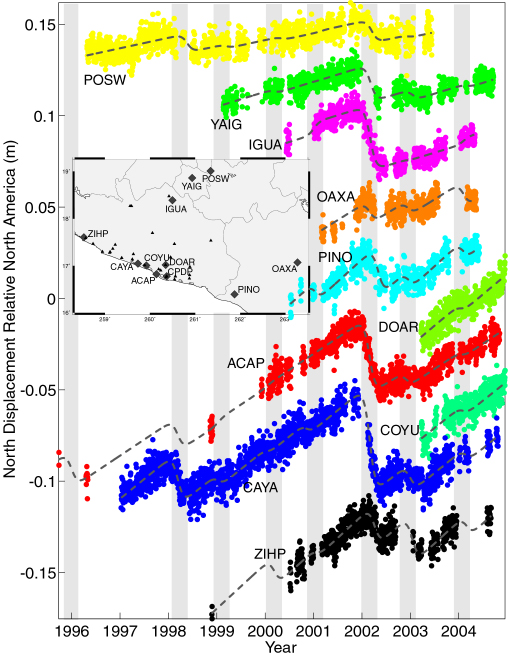
Unfortunately, campaign data from Guerrero were collected before the possibility of transient deformation had been recognized. Transients are evident in 1996, 1998, 1999, 2000, 2001, 2002, 2003 and 2004, from campaign data collected in 1992, 1995, 1996, 1998, 2000 and 2001. The first continuous GPS site began measurement in 1996, a second in 1997, and most of the rest of the continuous sites were installed in 1999, 2000, or 2003. Not all campaign sites were occupied at all epochs, and only one site (ACAP) was sampled sufficiently to separate all of the eight recognized transients from the steady-state site velocity. Guerrero state is just one of many subduction zones where tens to hundreds of thousands of dollars were spent to collect campaign GPS measurements before continuous GPS measurements indicated transient slip behavior. Ideally, we would like to make use of these early data rather than to simply discard them.
Squeezing More from the Data:
Modeling the displacement time series at a particular site requires (at a minimum) two parameters to describe the steady-state slope and intercept plus one parameter to describe the total displacement during each transient event. However, our data are not adequate to separate steady-state from transients at many of the sites. To circumvent this problem, we recognize that (1) total deformation between any two sampling epochs must equal the sum of steady-state for that period plus any transient displacements, and (2) displacements and/or velocities due to deep slip must be very similar at closely-spaced sites. Hence we can substitute spatial redundancy for temporal redundancy at some campaign sites.
I model steady-state velocity as spatially variable coupling between the Cocos and North American plates. (A more detailed description of the steady-state slip modeling is given in Larson et al. [2004]). The coupling model can be thought of as a smooth interpolator of steady-state velocity estimates from well-sampled sites to poorly-sampled sites that enables a more robust estimate of transient displacement at those sites. The velocity field from steady-state coupling must vary smoothly because surface deformation has a spatial wavelength roughly twice the depth of the source, and the Guerrero plate interface is deep (ranging from 20 km depth at the coast to more than 80 km below inland sites such as IGUA and YAIG). Consequently, closely-spaced GPS sites must have very similar steady-state velocities and similar transient displacements.
Transient slip is modeled in two very different ways to provide a sense of the range of possible solutions. In one model, I assume slip is uniform within a single rectangular region or patch on the plate boundary, and solve via grid search for the length, width, location, slip and timing parameters that best fit the GPS data. A more detailed description of this approach is given here and in Larson et al. [2004]. In the second modeling approach, I solve for variable slip on a discretized representation of the plate boundary and limit the solution space by requiring that the slip in each event is less than the slip deficit accumulated by frictional coupling (minus transient slip) since the beginning of GPS observation. A more detailed description of the discretized modeling approach, and a comparison of the two modeling approaches, is given in Lowry et al. [2005]. In general, constraints on the discretized model force smaller slip (and hence smaller moment release) in each event, and discretized models locate slip nearer to the GPS sites (which are situated predominantly on the Guerrero coastline).
Best-fit models of steady-state slip are given here for both the
single patch 
| and discretized 
|
Best-fit results of both the single patch and discretized models of transient slip are also given for each of the
1996,
|
|
1998,
|
|
1999,
|
|
2000,
|
|
2001,
|
|
2002,
|
|
2003,
|
|
and 2004
|
|
An alternative inverse solution, in which coseismic displacements during earthquakes are modeled and removed prior to inverting for transient and steady-state slip, is given here for the 1992-2001 period only. The results are quite similar with and without the inclusion of displacement models for earthquakes other than the 1995 Mw=7.3 Copala event. Slip during the Copala earthquake is treated as an unknown parameter to be solved for in each model.
Time series of GPS positions, corrected for rigid rotation of the North American plate, are also shown for each of the sites relative to MDO1 and/or ACAP below. Red circles are daily coordinate solutions with 95% confidence indicated by cyan bars. Blue represents the best-fit model from inversion, and yellow indicates the periods of transient episodes.